Why Vanilla RNNs Struggle with Sequence Problems

Why Vanilla RNNs Struggle with Sequence Problems

A beginner-friendly guide to understanding RNNs, their limitations.

1. What Is a Sequence Problem?

In real life, many problems aren’t just about data, they are about order.

A sequence problem is one where what comes before directly affects what comes next. If you change the order, you change the meaning.

Simple Examples:

• Sentences: "I am not happy" vs. "I am happy." The order of words is everything.

• Time Series: Yesterday’s stock price influences today's price.

• DNA: The specific order of genes determines biological function.

In one Line: "A sequence problem is where the history of the data is just as important as the data itself."

2. Where Do We See Sequence Problems?

We use models to solve these daily in various domains:

• NLP (Text): Translation (English to French), sentiment analysis (Is this review positive?), and chatbots.

• Time Series: Weather forecasting, stock market trends, and predicting ATM cash needs.

• Speech: Converting audio signals into text.

• Bioinformatics: Reading DNA and protein sequences.

3. Why Normal Neural Networks Fail

Traditional neural networks (like feedforward networks) have a major flaw: They have no memory.

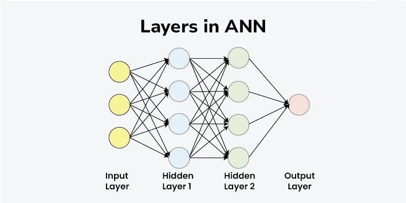
Imagine reading a movie review: "The movie was very long but amazing." A normal network looks at the word "amazing" in isolation. It has already forgotten that the sentence was talking about a "movie." To understand language or trends, we need a network that remembers.

4. What Is an RNN?

A Recurrent Neural Network (RNN) is a neural network with a "notebook."

As it reads data step-by-step, it keeps a Hidden State or Memory (ht). It reads a word, writes a note in its notebook, and carries that notebook to the next word.

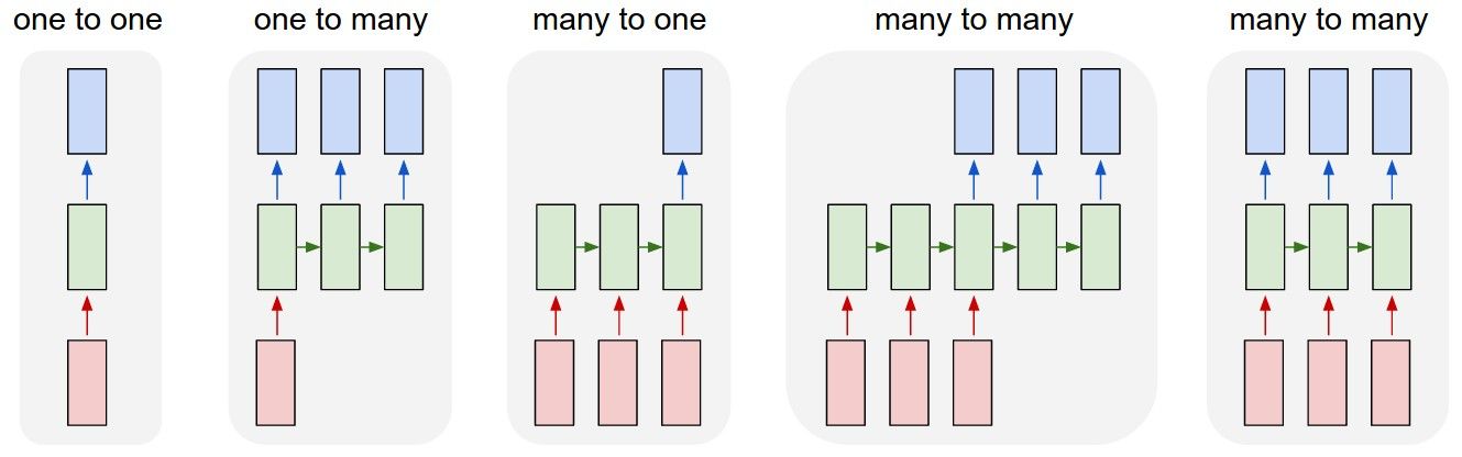
The Taxonomy of RNNs

Depending on the task, we use different "shapes" of RNNs to handle these sequences:

1. One-to-Many: A single input produces a sequence of outputs.

(Example: Image Captioning.)

2. Many-to-One: A sequence of inputs results in a single output.

(Example: Sentiment Analysis.)

3. Many-to-Many (Synchronous): The input and output sequences have the same length and happen simultaneously.

(Example: Named Entity Recognition.)

4. Many-to-Many (Asynchronous): Also known as the Encoder-Decoder or Seq2Seq model. This was formalized in the seminal work by Sutskever et al. (2014) (1409.0473). The model reads the entire input sequence before it starts producing an output sequence of a potentially different length.

(Example: Machine Translation.)

The Simple "Math":

Take the sentence “Cryptocurrency is the next big thing”. At time t1 “Cryptocurrency” will be fed into the network, at time t2 “is” be fed into the network, at time t3 “the” be fed into the network, and so forth.

Input data format:

Input data = (time steps, input features)

1. Time Steps (Sequence Length): The number of elements in the sequence, such as the number of words in a sentence or historical data points in a time series.

2. Input Features: The dimensionality of each element at a single time step, such as a 100D word embedding or a single numerical value for a univariate time series.

We denote a hidden state using this formula:

hₜ = tanh(Wₕhₜ₋₁ + Wₓxₜ)

When t = 1,
h₁ = tanh(Wₕh₀ + Wₓx₁), where x₁ is ‘Cryptocurrency’, and h₀ is initialized as zero.

When t = 2,
h₂ = tanh(Wₕh₁ + Wₓx₂), where x₂ is ‘is’.

When t = 3,
h₃ = tanh(Wₕh₂ + Wₓx₃), where x₃ is ‘the’.

Translation: Your current memory is a mix of what you just saw and what you already knew.

The weight parameters for both hidden state and input are learnable, which means that during the training it will update itself using backpropagation.

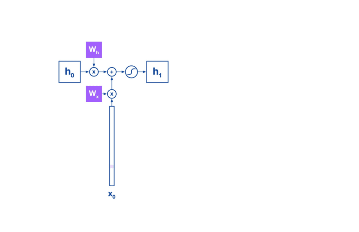
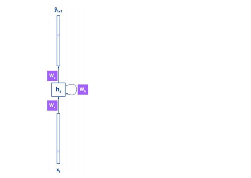
If you notice the formula above you will observe that the parameters ={Wh,Wx,Wy} remain constant in each and every input. This is known as parameter sharing. Parameter sharing gives RNNs the ability to structure and retain contextual information even if the length of the sentence has variable length. Such sharing is important when we want to model a sequence where a data can reoccur quite often. RNNs share the same weight across several time steps.

Training RNNs

Computing gradients: Backpropagation through time

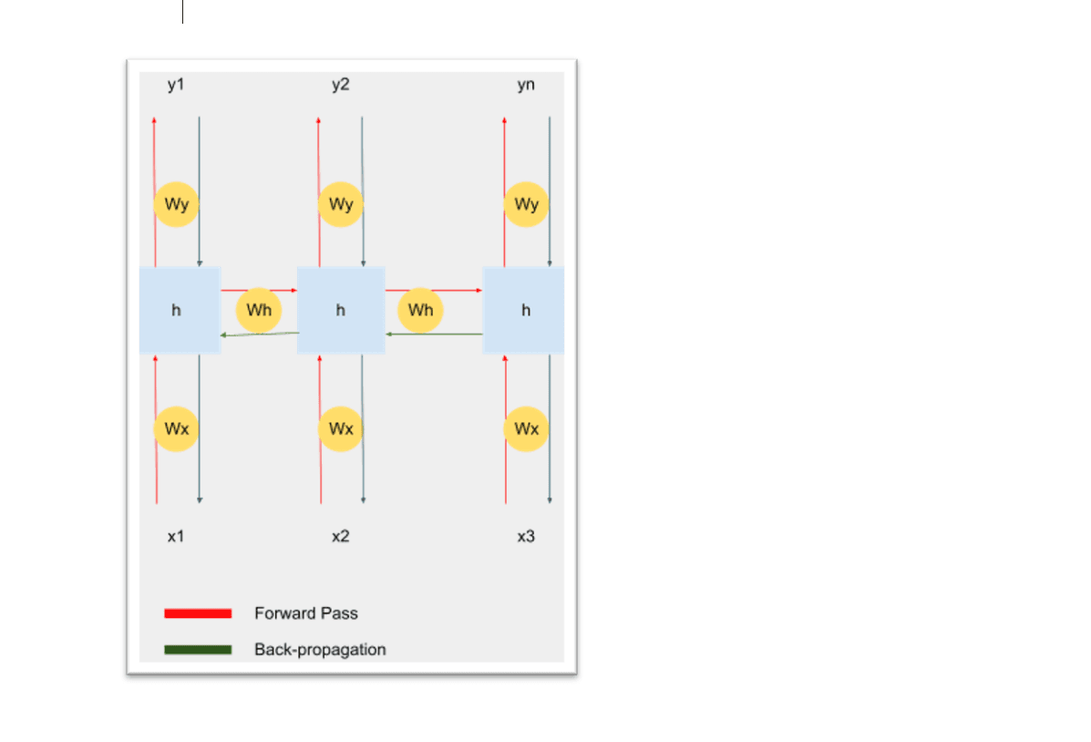
So far we’ve seen how feed-forward works in RNNs, i.e. the inputs enter the network and move forward while sharing the same parameter across each time step. During backpropagation it has to go back through the time-step to update the parameters.

So how does it happen?

Predicting output in RNN is a classification task, so we use cross-entropy to calculate the loss.

L₀(y, y′)ₜ = −yₜ log y′ₜ

Where θ = {Wₕ, Wₓ, Wᵧ}

yₜ = softmax(Wᵧ hₜ)

We know that the parameters are shareable, and it’s this ability of RNNs that makes all the difference in the network; it’s quite tricky to differentiate. In order to tackle this problem, the network needs to be expanded, or unfolded, so that the parameters could be differentiated across the network with respect to time step, hence the term backpropagation through time (BPTT).

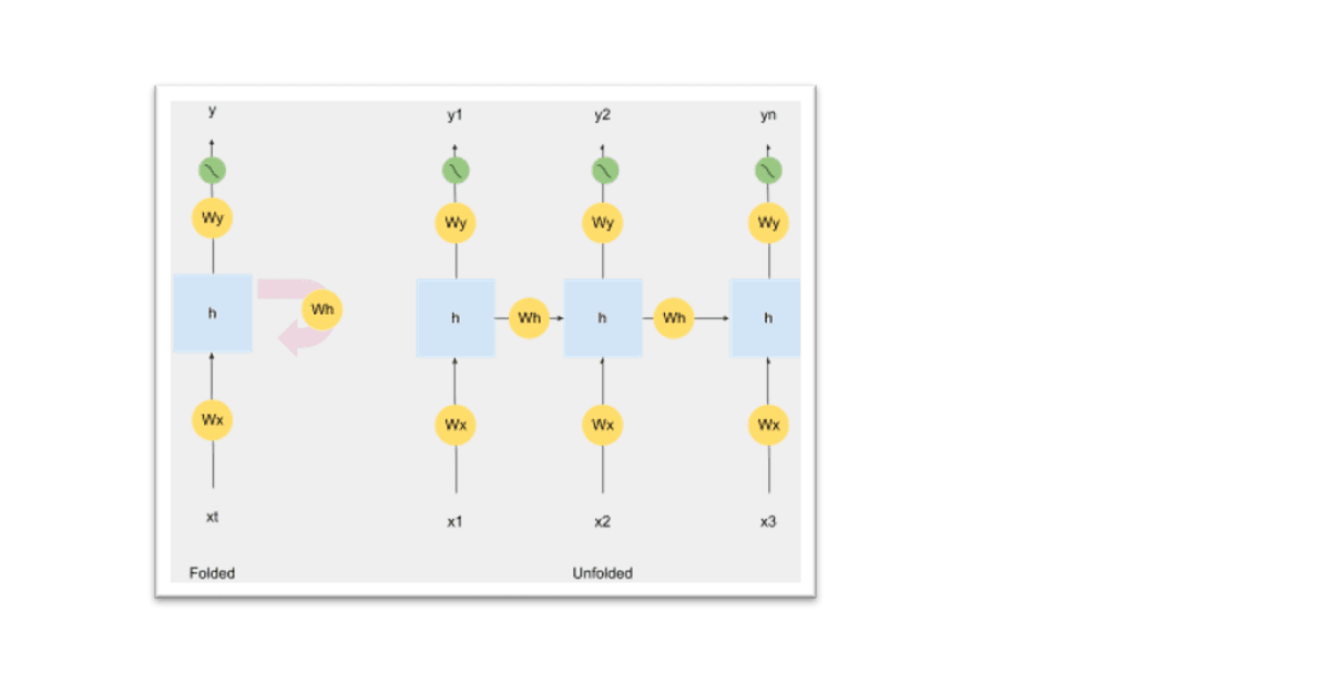
From the above diagram you can see how an unfolded recurrent network looks like.

Since the neural network takes one word at a time, the loss calculated is based on per-word basis. The overall procedure looks like this:

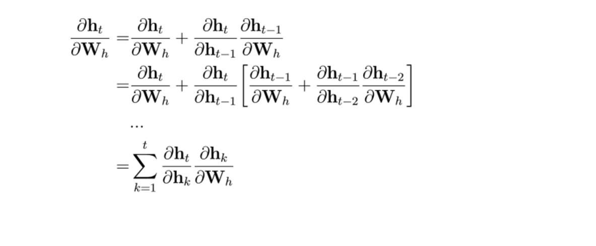
You can see how the expansion in formula takes place.

For differentiation with respect to Wy, the procedure should look like this:

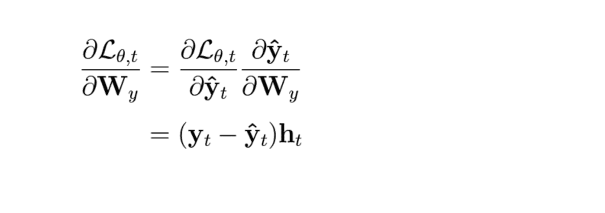
So, let’s summarize backpropagation:

1. Loss is computed using the current output and the actual output using cross-entropy loss

2. The network is unrolled, or expanded, so that the backpropagation could take place through hidden layers and also through time

3. The weights parameters are updated for both recurrent neuron, i.e. hidden state, and the dense layers

Sudo Code

rnn = RNN()
y = rnn.step(x)  # x is an input vector, y is the RNN's output vector

class RNN:
  # ...
  def step(self, x):
    # update the hidden state
    self.h = np.tanh(
        np.dot(self.W_hh, self.h) +
        np.dot(self.W_xh, x)
    )
    # compute the output vector
    y = np.dot(self.W_hy, self.h)
    return y

PyTorch Code

import torch.nn as nn

# A simple RNN in PyTorch
# input_size: number of features (e.g., 100D word embedding)
# hidden_size: the size of our "notebook" or memory

rnn = nn.RNN(
    input_size=10,
    hidden_size=20,
    batch_first=True
)

Where RNNs Actually Work Well

Vanilla (simple) RNNs are not useless! They are actually quite efficient for:

• Short sentences: "How are you?"

• Simple patterns: Short-term weather changes.

• Small datasets: Where dependencies are very close to each other.

The problem:

Issues with gradients

Two common problems that occur during the backpropagation of sequential data are vanishing and exploding gradients.

Vanishing gradients

When the differentiating vector goes to zero exponentially fast, which in turn makes it difficult for the network to learn some long period dependencies, the problem is vanishing gradient.

Coming to backpropagation in RNNs, we saw that every single neuron in the network participated in the calculation of the output with respect to the cost function. Because of that, we have to make sure that the parameters are updated for every neuron to minimize the error, and this goes back to all the neurons in time. So, you have to propagate all the way back through time to these neurons.

We also know that the contextual vector, or the hidden state parameter, is shared across the network to preserve order and continuity. During initialization, the parameter is assigned with a random number which is close to zero, and when the hidden state moves forward in time it gets multiplied by itself over at different time steps, making the gradient Wh smaller and smaller, essentially zero to a point where it vanishes.

The lower the gradient is, the harder it is for the network to update the weights, and if the gradient is zero, the weights will not be updated.

Exploding gradients

Exploding gradients occur when large gradients accumulate due to an unstable process, and result in very large updates to the parameters.

In RNNs, exploding gradients can occur during backpropagation and result in very large gradients essentially making large updates to the network parameters. At an extreme, the values of weights can become so large that they become NaN values.

Overcoming gradient issues

Gradient issues in RNNs can be solved with:

• Gated networks

5. Long Short Term Memory (LSTM)

Long short term memory was built to preserve long term contextual information of a sequence that the RNN lacks.

The core idea of LSTM is to make sure the gradient flows for a long period of time, and doesn’t vanish or explode.

As we saw earlier, RNNs have a standard architecture where the hidden state formed some sort of a looping mechanism to preserve and share the information for every time step. Well, LSTM also has a looping mechanism. Instead of having a single neural network layer, there are four neural networks, interacting in a way to preserve and share long contextual information.

Let’s understand how the LSTM network works step-by-step:

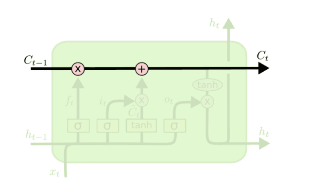
1. Cell state:

The long-term memory is usually called the cell state, denoted by Ct-1, and recursive in nature. Cell state allows previous information to be stored in the LSTM network. It’s modulated by the internal gates namely: forget and input gate.

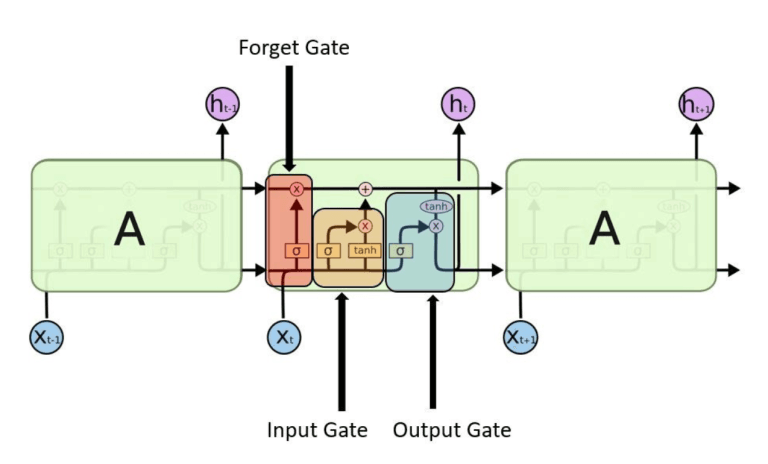
2. Forget gate:

The cell state is connected to the forget gate which dictates which information to preserve and which to forget. It does this through a sigmoid function. It looks at the initial state at ht-1 and xt, and outputs a number between 0 and 1 for each cell state Ct-1. If the information returned by the forget gate is 1, it stores the information, and if it returns 0, it deletes the information.

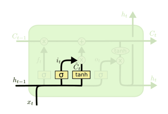
3. Input gate:

The input gate takes the same input xt from the same initial state ht-1 and it passes through two non-linear activation functions: sigmoid (which returns the value between 0 and 1) and tanh (which returns the value between -1 and 1), which are input gate and candidate memory Ct. This helps the cell state to save new information and simultaneously update the cell state from Ct-1 to Ct. The idea of the input gate is to store new information in the cell state, along with the pruned memory from the forget gate.

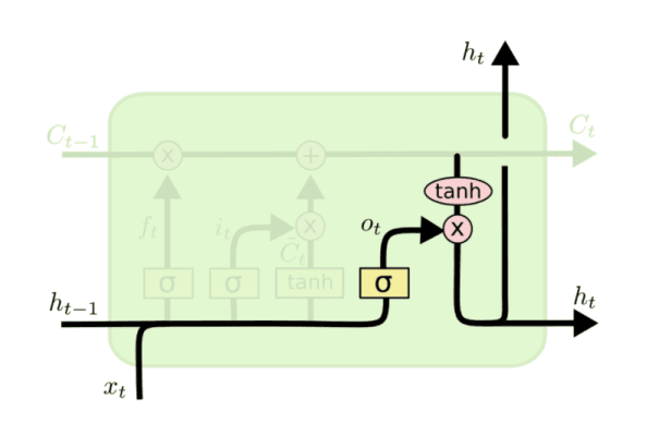
4. Output gate:

The output will be based on the cell state Ct, the initial hidden state ht-1and input xt. The hidden state and input will be passed through a sigmoid so that value is between 0 and 1. Simultaneously we pass cell state Ct through the tanh to get values between 1 and -1, and multiply it by the output of the sigmoid gate, so that we only output what’s relevant to the context.

At glance

1. The first sigmoid activation function is the forget gate that ensures what information should be forgotten from the previous cell state (Ct-1).

2. The second sigmoid and first tanh activation function is for the input gate that ensures what information should be saved to the cell state along with the previous pruned information.

3. The last sigmoid is the output gate and tanh from the cell that highlights which information should be going to the next hidden state.

PyTorch LSTM Example

import torch
import torch.nn as nn

# Define an LSTM layer
lstm = nn.LSTM(
    input_size=10,
    hidden_size=20,
    batch_first=True
)

# The output now includes both the Hidden State (h) and the Cell State (c)
# Cell State (c) acts like a "conveyor belt" of long-term memory

output, (h_n, c_n) = lstm(input_data)

Explanation

• output → Output features from the LSTM for each time step
• h_n (Hidden State) → Final hidden state for each layer
• c_n (Cell State) → Final cell state carrying long-term memory

6. Encoder-decoder sequence-to-sequence architecture

The advantage of using RNNs in sequential modeling is that it can:

• Map an input sequence to a fixed-size vector

• Map fixed-size vector to a sequence

• Map an input sequence to an output sequence of the same length.

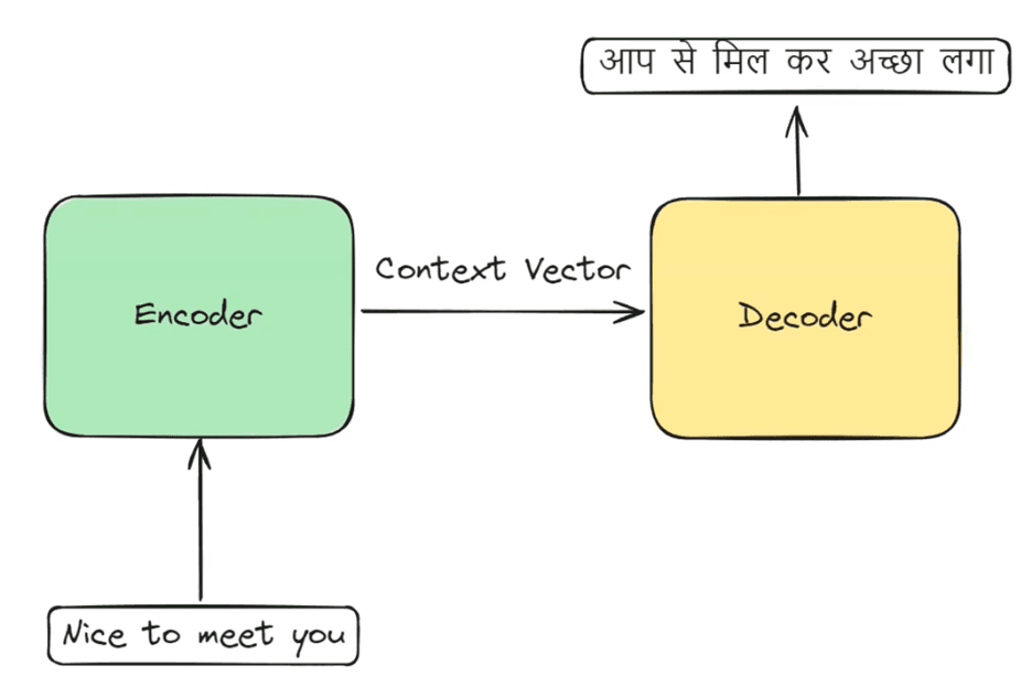
But let’s say we want to train a RNN to map an input sequence to an output sequence, not necessarily of the same length. This can come up especially when we want to translate from one language to another.

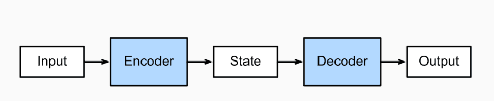
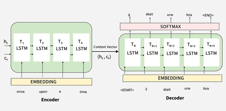
Encoder-decoder sequence-to-sequence is an architecture that deals with this type of problem. As the name suggests, it has two types of architecture: encoder and decoder.

Encoder RNN receives the input sequence of variable length, and processes it to return a vector or a sequence of vectors called the “context” vector C.

The decoder RNN is conditioned on a fixed-length vector to generate an output sequence. Also, the last hidden state of the encoder is the initial hidden state of the decoder.

7. The Solution: Attention

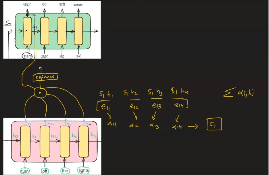
Attention was the breakthrough. It told the model: "Don't try to remember everything in one vector. Instead, when you translate a specific word, 'look back' at the most relevant words in the original sentence."

Analogy: Attention is like a highlighter. It highlights the important parts of the input so the model doesn't have to guess.

Phase 1: Bahdanau Attention (2014) – "The Additive Approach"

In the paper Neural Machine Translation by Jointly Learning to Align and Translate (1409.3215), Bahdanau et al. introduced the first iteration of Attention.

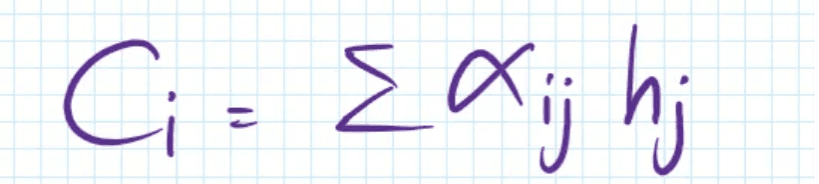
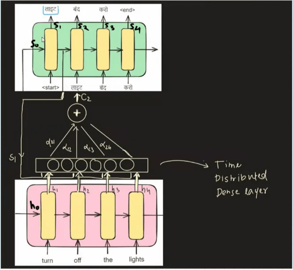
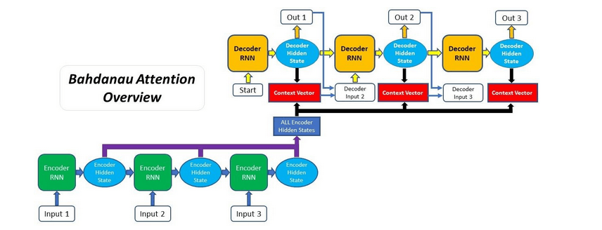
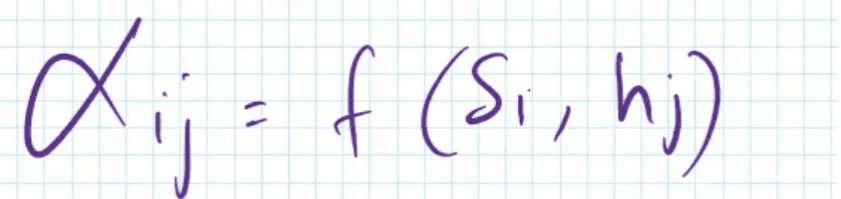
• The Logic: It uses a small neural network to calculate an "alignment score" between the current Decoder state and all the Encoder's hidden states.

• The Math (Additive): It "adds" the information of the Decoder and Encoder together and passes it through a tanh activation function to determine which parts of the input are relevant right now.

• The Limitation: Because it uses a separate neural network layer to calculate every single attention score, it is computationally expensive.

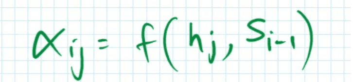
The function f() = Artificial Neural Network (ANN) acts as a Universal Approximation Function

Phase 2: Luong Attention (2015) – "The Multiplicative Refinement"

A year later, in Effective Approaches to Attention-based Neural Machine Translation (1508.04025), Luong et al. simplified the process.

• The Logic: Instead of a complex additive network, why not use the Dot Product? The dot product is a mathematical way of asking: "How similar are these two vectors?"

• The Math (Multiplicative): You simply multiply the Decoder state by the Encoder states.

• The Benefit: It is much faster and more memory-efficient. This "Dot-Product Attention" paved the way for massive scaling.
  
  
  
  

Feature	Bahdanau (2014)	Luong (2015)
Math Type	Additive (concat + linear)	Multiplicative (dot product)
Complexity	High	Low (Fast)
Alignment	Uses previous decoder state	Uses current decoder state

8. Implementation of RNN in Keras / Tensorflow and Python

Importing required libraries

import numpy as np

from tensorflow.keras.layers.recurrent import SimpleRNN
from tensorflow.keras.models import Sequential
from tensorflow.keras.layers import Dense, Activation

You can download the dataset here.

INPUT_FILE = "data/wonderland.txt"

Data preprocessing

Data preprocessing is needed because the data contains ASCII characters, which might interfere with our modeling process and give incorrect results.

print("Extracting text from input")

file = open(INPUT_FILE, 'rb')
lines = []

for line in file:
    line = line.strip().lower()
    line = line.decode("ascii", "ignore")
    if len(line) == 0:
        continue
    lines.append(line)

file.close()
text = " ".join(lines)

After the data is cleaned, we can create a look-up table. The look-up table basically creates a table of unique characters from the data. This table will convert the characters in the text to numbers, which will then be fed into the RNNs.

chars = set([c for c in text])
nb_chars = len(chars)

char2index = dict((c, i) for i, c in enumerate(chars))
index2char = dict((i, c) for i, c in enumerate(chars))

print(index2char)

Output:

{
 0: '!',
 1: 's',
 2: '7',
 3: 'p',
 4: 'x',
 5: '.',
 6: ']',
 7: '3',
 8: 'a',
 9: 'z',
 10: '9',
 11: '5',
 12: '6',
 13: 'h',
 14: ',',
 15: 'c',
 16: 'r',
 17: '@',
 18: 'k',
 19: 'w',
 20: 'd',
 21: '(',
 22: 'o',
 23: 'f',
 ...
}

Now, we’ll create inputs and labels. It’s important to understand that in sequence modeling, the input will start from index 0, where the label will start from index 1.

For instance, if we feed “cryptocurrency is the next big thing”, then:

Input	Label
cryptocurrency	is
is	the
the	next
next	big
big	thing
thing

*It’s worth mentioning that it’s a character level RNN, so instead of words you will be working with characters.

print("Creating input and label")

SEQ_LEN = 10
STEP = 1

print("The table is ready")

input_chars = []
label_chars = []

for i in range(0, len(text) - SEQ_LEN, STEP):
    input_chars.append(text[i:i + SEQ_LEN])
    label_chars.append(text[i + SEQ_LEN])

print(input_chars)

Output:

[
 'project gu',
 'roject gut',
 'oject gute',
 'ject guten',
 'ect gutenb',
 'ct gutenbe',
 't gutenber',
 ' gutenberg',
 'gutenbergs',
 ...
]

One-hot encoding

Transforming sequences to one-hot-encoded vectors.

print("Vectorizing input and label text...")

X = np.zeros((len(input_chars), SEQ_LEN, nb_chars), dtype=np.bool)
y = np.zeros((len(input_chars), nb_chars), dtype=np.bool)

for i, input_char in enumerate(input_chars):
    for j, ch in enumerate(input_char):
        X[i, j, char2index[ch]] = 1
    y[i, char2index[label_chars[i]]] = 1

Modeling the RNN

Defining the model:

• RNN will contain 128 hidden states

• Always remember that the dense layer should equal the number of unique characters in the text

RNN Model Configuration & Training

HIDDEN_SIZE = 128
BATCH_SIZE = 128
NUM_ITERATIONS = 25
NUM_EPOCHS_PER_ITERATION = 1
NUM_PREDS_PER_EPOCH = 100

# Build the RNN model
model = Sequential()
model.add(
    SimpleRNN(
        HIDDEN_SIZE,
        return_sequences=False,
        input_shape=(SEQ_LEN, nb_chars),
        unroll=True
    )
)
model.add(Dense(nb_chars))
model.add(Activation("softmax"))

# Compile the model
model.compile(
    loss="categorical_crossentropy",
    optimizer="rmsprop"
)

Training the Model

for iteration in range(NUM_ITERATIONS):
    print("=" * 50)
    print("Iteration #: %d" % (iteration))

    model.fit(
        X,
        y,
        batch_size=BATCH_SIZE,
        epochs=NUM_EPOCHS_PER_ITERATION
    )

    # testing model
    # randomly choose a row from input_chars, then use it to 
    # generate text from model for next 100 chars

    test_idx = np.random.randint(len(input_chars))
    test_chars = input_chars[test_idx]

    print("Generating from seed: %s" % (test_chars))
    print(test_chars, end="")

    for i in range(NUM_PREDS_PER_EPOCH):
        Xtest = np.zeros((1, SEQ_LEN, nb_chars))

        for j, ch in enumerate(test_chars):
            Xtest[0, j, char2index[ch]] = 1

        pred = model.predict(Xtest, verbose=0)[0]
        ypred = index2char[np.argmax(pred)]

        print(ypred, end="")

        # Move the sliding window forward
        test_chars = test_chars[1:] + ypred

    print()

9. Conclusion & What's Next

We've come a long way:

1. RNNs gave us memory.

2. LSTMs gave us long-term memory.

3. Attention gave us focus.

But one problem remains: Even with Attention, LSTMs are still sequential (word-by-word). They are still slow.

To solve speed and long-range memory at the same time, we need a model that doesn't read word-by-word at all. That is where Self-Attention and Transformers come in.

Stay tuned for the next article where we dive into the world of Transformers!

References & Deep Dives

• RNN → https://jontalle.web.engr.illinois.edu/Public////Elman-FindingStructureinTime.90.pdf

• LSTM → https://ieeexplore.ieee.org/abstract/document/6795963

• Seq2Seq → https://arxiv.org/abs/1409.0473

• Bahdanau Attention → https://arxiv.org/abs/1409.3215

• Luong Attention → https://arxiv.org/abs/1508.04025